Base class representing a spectral image. More...
#include <SpecImage.hpp>
Public Member Functions | |
| SpecImage () | |
| Default constructor. More... | |
| SpecImage (const csr_mat_t< FPType > &matrix, const FPType *mzvals=NULL) | |
| Constructor: construct a nag::SpecImage object from a sparse matrix and optionally provide m/z values. More... | |
| SpecImage (size_t m, size_t n, const FPType *matrix, const FPType *mzvals=NULL) | |
| Constructor: construct a nag::SpecImage object from a dense column-major matrix and optionally provide m/z values. More... | |
| virtual | ~SpecImage () |
| Destructor. More... | |
| void | peakSelect () |
| Perform peak selection. More... | |
| pca_results_t< FPType > | pca (uint32_t k, pca_mat_t t=Covariance) |
| Principal component analysis. More... | |
| kmeans_results_t< FPType > | kmeans (uint32_t k, FPType *initial_cmeans=NULL, kmeans_metric_t metric=Cosine) |
| k-means clustering analysis More... | |
| nmf_results_t< FPType > | nmf (uint32_t k, FPType *initial_W=NULL, FPType *initial_H=NULL, FPType tol=1.e-2, uint32_t max_iter=200) |
| Non-negative matrix factorization. More... | |
| cwt_results_t< FPType > | cwt (const std::vector< uint32_t > &scales, const std::vector< size_t > &pixels, wavelet_t wav=Haar, wavelet_extension_t ext=Periodic) |
| Batched one-dimensional real continuous wavelet transform. More... | |
| tsne_results_t< FPType > | tsne (uint32_t k, pca_results_t< FPType > *data=NULL, FPType *embedding=NULL, FPType perplexity=50, FPType theta=0.3, uint32_t max_iter=1000, uint32_t verbosity=50, FPType min_grad_norm=1.0e-5, uint32_t n_unimproved_iter=30, FPType learning_rate=100, FPType early_exaggeration=4.0, uint32_t exaggerated_iter=50) |
| t-SNE analysis More... | |
| csr_mat_t< FPType > | getSparseMatrix (matrix_ordering_t order=PixelsByChannels) |
| Retrieve a copy of the image matrix in sparse storage format. More... | |
| std::unique_ptr< FPType[]> | getDenseMatrix (matrix_ordering_t order=PixelsByChannels) |
| Retrieve a copy of the image matrix in dense storage format. More... | |
| std::vector< FPType > | getSinglePeak (FPType minmz, FPType maxmz) |
| Return a single peak. A lower limit minmz and an upper limit maxmz are used to reduce the number of channels (columns) in the image matrix to 1. The original image matrix is left unchanged when the single channel is extracted. This allows multiple peaks of interest to be quickly investigated before final peak selection is performed on the data. More... | |
| size_t | getM () |
| Return the number of rows in the matrix. More... | |
| size_t | getN () |
| Return the number of columns in the matrix. More... | |
| size_t | getNNZ () |
| Return the number of non-zero elements in the matrix. More... | |
| int | getXDim () |
| Return the number of pixels in the image in the \(x\) dimension. More... | |
| int | getYDim () |
| Return the number of pixels in the image in the \(y\) dimension. More... | |
| int | getZDim () |
| Return the number of pixels in the image in the \(z\) dimension. More... | |
| std::vector< FPType > | getMZVals () |
| Return the mass-to-charge values which label the channels in the image matrix. More... | |
| void | setLimits (const std::vector< FPType > &limits) |
| Set the limits to use during nag::SpecImage::peakSelect. More... | |
| source_t | getSource () |
| Determine the type of the object. More... | |
Protected Attributes | |
| void * | _imgh |
| Opaque handle to internal library data structure. More... | |
| source_t | _source_type |
| Encodes what the underlying type is: nag::SIMSpecImage (value: SIMS), nag::MALDISpecImage (value: MALDI) or nag::SpecImage (value: none). More... | |
Detailed Description
template<class FPType>
class nag::SpecImage< FPType >
Base class representing a spectral image.
Constructor & Destructor Documentation
|
inline |
Default constructor.
| nag::SpecImage< FPType >::SpecImage | ( | const csr_mat_t< FPType > & | matrix, |
| const FPType * | mzvals = NULL |
||
| ) |
Constructor: construct a nag::SpecImage object from a sparse matrix and optionally provide m/z values.
- Parameters
-
[in] matrix The sparse matrix to copy. [in] mzvals The mzvals array to use. The length of this array must match the number of columns of matrix.
| nag::SpecImage< FPType >::SpecImage | ( | size_t | m, |
| size_t | n, | ||
| const FPType * | matrix, | ||
| const FPType * | mzvals = NULL |
||
| ) |
Constructor: construct a nag::SpecImage object from a dense column-major matrix and optionally provide m/z values.
- Parameters
-
[in] m The number of rows of the matrix. [in] n The number of columns of the matrix. [in] matrix The dense matrix to copy, in column-major storage. [in] mzvals The mzvals array to use. The length of this array must match the number of columns of matrix, n.
|
virtual |
Destructor.
Member Function Documentation
| cwt_results_t<FPType> nag::SpecImage< FPType >::cwt | ( | const std::vector< uint32_t > & | scales, |
| const std::vector< size_t > & | pixels, | ||
| wavelet_t | wav = Haar, |
||
| wavelet_extension_t | ext = Periodic |
||
| ) |
Batched one-dimensional real continuous wavelet transform.
A continuous wavelet transform
\[C_{s,k} = \int x(t)\frac{1}{\sqrt{s}}\psi^*(\frac{t - k}{s})dt\]
is defined over a signal \(x(t)\) at scale \(s\) and position \(k\) using the mother wavelet \(\psi(t)\).
Here, the input signal \(x(t)\) is a pixel's spectrum, and the above transform is typically performed over a number of different scales, producing a matrix of transformation coefficients \(C_{s,k}\) for each pixel.
The transformation is a convolution of the selected mother wavelets, scaled, with the input \(x(t)\), producing coefficients with a high value where the input closely matches the scaled wavelet. Since wavelets are defined over a finite supporting domain, the coefficients give information about the characteristics of the input data within a locality.
We perform convolution using the circular convolution theorem, which states that the convolution of two finite sequences is equal to the inverse Fourier transform of the product of the forwards Fourier transforms. We thus replace the \(O(n^2)\) cost of direct convolution with \(O(n \log n)\) cost of the fast Fourier transform.
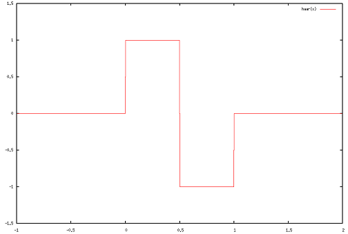
Two mother wavelets are provided in the cwt function: the Haar wavelet and the Mexican Hat. The Haar wavelet is defined as follows:
\[\psi(x) = \begin{cases} 1 \quad & 0 \leq x < \frac{1}{2},\\ -1 & \frac{1}{2} \leq x < 1,\\ 0 &\mbox{otherwise.}\end{cases}\]
It is supported (i.e. is non-zero) over [0,1):
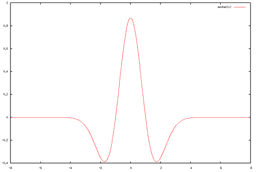
The Mexican Hat wavelet is defined as:
\[\psi(x) = \frac{2}{\sqrt{3}\pi^{1/4}} (1 - x^2)e^{(-x^2/2)}.\]
It is supported over [-8, 8] (using a conservative truncation):
In addition to selecting a mother wavelet it is also possible to select how the ends of the input are handled. There are 3 options: zero end extension (points beyond the ends are taken to be zero), symmetric end extension (values are reflected so that \(x_{-1} = x_0, x_{-2} = x_1, x_{-3} = x_2\) etc. and \(x_n = x_{n-1}, x_{n+1} = x_{n-2}, x_{n+2} = x_{n-3}\) etc.) or periodic end extension ( \(x_{-1} = x_{n-1}, x_{-2} = x_{n-2}\) etc. and \(x_n = x_0, x_{n+1} = x_1\) etc.).
- Parameters
-
[in] scales The scales to use in the transform. [in] pixels The pixels to be transformed. Note that pixels are numbered from zero, and are taken to be contiguous in x, then y, then z. E.g. to find the index of pixel \((x,y,z)\) in a 1-based coordinate system with \(X\), \(Y\), \(Z\) pixels in the respective dimensions: \(pixel = X\times Y\times (z - 1) + X\times (y - 1) + x - 1\). [in] wav The mother wavelet to use in the transform: nag::Haar or nag::MexicanHat. [in] ext The end extension to use in the transform: nag::Periodic, nag::Zero or nag::Symmetric.
| std::unique_ptr<FPType[]> nag::SpecImage< FPType >::getDenseMatrix | ( | matrix_ordering_t | order = PixelsByChannels | ) |
Retrieve a copy of the image matrix in dense storage format.
- Parameters
-
[in] order Determines whether pixels are represented by columns or rows in the returned matrix. If order is nag::PixelsByChannels then each row of the matrix holds a pixel's spectrum; if order is nag::ChannelsByPixels then each column of the matrix holds a pixel's spectrum. Note that pixels are numbered from zero, and are taken to be contiguous in \(x\), then \(y\), then \(z\). E.g. to find the index of pixel \((x,y,z)\) in a 1-based coordinate system with \(X\), \(Y\), \(Z\) pixels in the respective dimensions: \(pixel = X\times Y\times (z - 1) + X \times (y - 1) + x - 1\).
- Returns
- A pointer to the dense matrix stored in column-major ordering. The dimensions of the matrix can be found by calling nag::SpecImage::getM (the number of rows) and nag::SpecImage::getN (the number of columns).
| size_t nag::SpecImage< FPType >::getM | ( | ) |
Return the number of rows in the matrix.
This corresponds to the number of pixels in the image matrix. Note that pixels are numbered from zero, and are taken to be contiguous in \(x\), then \(y\), then \(z\). E.g. to find the index of pixel \((x,y,z)\) in a 1-based coordinate system with \(X\), \(Y\), \(Z\) pixels in the respective dimensions: \(pixel = X\times Y\times (z - 1) + X\times (y - 1) + x - 1\).
| std::vector<FPType> nag::SpecImage< FPType >::getMZVals | ( | ) |
Return the mass-to-charge values which label the channels in the image matrix.
The vector returned is of length \(n\), the number of channels in the image matrix.
| size_t nag::SpecImage< FPType >::getN | ( | ) |
Return the number of columns in the matrix.
This corresponds to the number of channels in the image matrix. The channels are labelled by mass-to-charge (m/z) values, which are held in an array of length \(n\). See nag::SpecImage::getMZVals.
| size_t nag::SpecImage< FPType >::getNNZ | ( | ) |
Return the number of non-zero elements in the matrix.
| std::vector<FPType> nag::SpecImage< FPType >::getSinglePeak | ( | FPType | minmz, |
| FPType | maxmz | ||
| ) |
Return a single peak. A lower limit minmz and an upper limit maxmz are used to reduce the number of channels (columns) in the image matrix to 1. The original image matrix is left unchanged when the single channel is extracted. This allows multiple peaks of interest to be quickly investigated before final peak selection is performed on the data.
- Parameters
-
[in] minmz The lower m/z limit to use for the channel. [in] maxmz The upper m/z limit to use for the channel.
- Returns
- A vector consisting of the single column (in dense format) of the matrix crresponding to the selected peak.
|
inline |
Determine the type of the object.
This function may be used to determine the inherited type of the object.
If this function returns nag::SIMS then the object is of type nag::SIMSpecImage and the data was generated by a SIMS instrument.
If it returns nag::MALDI then the object is of type nag::MALDISpecImage and the data was generated by a MALDI instrument.
If it returns nag::none then the object is of type nag::SpecImage.
| csr_mat_t<FPType> nag::SpecImage< FPType >::getSparseMatrix | ( | matrix_ordering_t | order = PixelsByChannels | ) |
Retrieve a copy of the image matrix in sparse storage format.
- Parameters
-
[in] order Determines whether pixels are represented by columns or rows in the returned matrix. If order is nag::PixelsByChannels then each row of the matrix holds a pixel's spectrum; if order is nag::ChannelsByPixels then each column of the matrix holds a pixel's spectrum. Note that pixels are numbered from zero, and are taken to be contiguous in \(x\), then \(y\), then \(z\). E.g. to find the index of pixel \((x,y,z)\) in a 1-based coordinate system with \(X\), \(Y\), \(Z\) pixels in the respective dimensions: \(pixel = X\times Y\times (z - 1) + X\times (y - 1) + x - 1\).
| int nag::SpecImage< FPType >::getXDim | ( | ) |
Return the number of pixels in the image in the \(x\) dimension.
Image dimensions returned are after any binning has been applied during construction of the image matrix.
| int nag::SpecImage< FPType >::getYDim | ( | ) |
Return the number of pixels in the image in the \(y\) dimension.
Image dimensions returned are after any binning has been applied during construction of the image matrix.
| int nag::SpecImage< FPType >::getZDim | ( | ) |
Return the number of pixels in the image in the \(z\) dimension.
Image dimensions returned are after any binning has been applied during construction of the image matrix.
| kmeans_results_t<FPType> nag::SpecImage< FPType >::kmeans | ( | uint32_t | k, |
| FPType * | initial_cmeans = NULL, |
||
| kmeans_metric_t | metric = Cosine |
||
| ) |
k-means clustering analysis
k-means clustering seeks to partition the pixels in the input matrix into a pre-defined number of clusters \(k\) such that the distance to the cluster mean is minimized. Each pixel is treated as an \(n\) dimensional vector, where \(n\) is the number of channels in the input matrix.
Two distance metrics are offered here: Euclidean distance and a distance based on cosine similarity, which we shall call cosine distance.
Euclidean distance between two vectors, \(\mathbf{a}\) and \(\mathbf{b}\), of length \(n\) is defined in the usual way:
\[\|\mathbf{a} - \mathbf{b}\|^2 = \sum_{i=1}^n (a_i - b_i)^2.\]
Cosine similarity is simply defined as the cosine of the angle between two vectors \(\mathbf{a}\) and \(\mathbf{b}\). Turning this into a distance metric, we define the cosine distance as:
\[D_c(\mathbf{a},\mathbf{b}) = 1 - \frac{\mathbf{a} \cdot \mathbf{b}}{\|\mathbf{a}\| \|\mathbf{b}\|}.\]
This is equivalent to Euclidean distance when the two vectors are normalized:
\[\| \mathbf{a} - \mathbf{b} \|^2 = \|\mathbf{a}\|^2 + \|\mathbf{b}\|^2 - 2\mathbf{a} \cdot \mathbf{b} = 2 - 2\mathbf{a} \cdot \mathbf{b} = 2D_c(\mathbf{a},\mathbf{b}).\]
Thus for the cosine distance option we work with normalized input and cluster means, and half of the distance defined above. Minimizing this distance function is equivalent to maximizing cosine similarity.
- Parameters
-
[in] k The number of clusters to find. [in,out] initial_cmeans If initial_cmeans is not NULL on entry the values supplied will be used as the initial cluster centroids, and on return will contain the computed k cluster centroids. If the parameter is NULL it is ignored and random initial cluster centroids will be used. [in] metric The metric to use - either nag::Euclidean or nag::Cosine.
| nmf_results_t<FPType> nag::SpecImage< FPType >::nmf | ( | uint32_t | k, |
| FPType * | initial_W = NULL, |
||
| FPType * | initial_H = NULL, |
||
| FPType | tol = 1.e-2, |
||
| uint32_t | max_iter = 200 |
||
| ) |
Non-negative matrix factorization.
Non-negative matrix factorization finds matrices \(W\), \(H\) which approximate an input matrix \(A\); that is \(A \approx WH\). Here \(A\) is the image matrix, where \(m\) is the number of pixels and \(n\) the number of channels.
If \(A\) is \(m\) by \(n\), then \(W\) is \(m\) by \(k\) and \(H\) is \(k\) by \(n\). \(k\) is typically selected such that \(k \ll min(m,n)\).
We use the alternating least-squares algorithm, which is an iterative procedure. In each iteration, a least-squares approximation to \(H\) is found, with \(W\) fixed:
\[ \underset{W >= 0}{arg\,min} \|WH - A\|^2.\]
All negative elements in \(H\) are then set to zero, before a least-squares approximation to \(W\) is found, with \(H\) fixed:
\[ \underset{H >= 0}{arg\,min} \|H^TW^T - A^T\|^2.\]
Finally all negative elements in \(W\) are set to zero.
We then normalize the rows of \(H\) and scale \(W\), using the scaling \(W = \dot{W}S\); \(H = S^{-1}\dot{H}\), where \(S\) is a diagonal matrix whose elements \(s_{ii}, i=1,\dots,k\) are the Euclidean norms of the \(i\)th row of \(H\), and \(\dot{W}\), \(\dot{H}\) represent the un-scaled solutions found by the least-squares algorithm, with negative elements replaced by zeroes.
We iterate until \(\|WH - A\|^2\) converges to within some tolerance, or a maximum number of iterations has been performed.
- Parameters
-
[in] k The inner dimension of the factorization: the number of columns of \(W\) and rows of \(H\). [in,out] initial_W If initial_W is not NULL on entry, the values supplied will be used as the initial values of the dense column-major \(m\) by \(k\) matrix \(W\), and on return will contain the computed \(W\). If initial_W is NULL, it is ignored and random initial values for \(W\) will be used. [in,out] initial_H If initial_H is not NULL on entry, the values supplied will be used as the initial values of the dense column-major \(k\) by \(n\) matrix \(H\), and on return will contain the computed \(H\). If initial_H is NULL it is ignored and random initial values for \(H\) will be used. [in] tol The convergence tolerance to use. [in] max_iter The maximum number of iterations to use.
| pca_results_t<FPType> nag::SpecImage< FPType >::pca | ( | uint32_t | k, |
| pca_mat_t | t = Covariance |
||
| ) |
Principal component analysis.
PCA is a technique used to find a new set of variables/axes for a multidimensional data set such that the new axes are mutually orthogonal and the greatest variance in the data occurs in the first axis, the next greatest in the second, and so on.
The new axes are called the PCA loadings and the projection of the data on to the loadings is the PCA scores.
In the PCA function provided here it is possible to select \(k\), the number of principal components to find, such that typically \(k \ll n\), where \(n\) is the number of variables (channels) in the image matrix.
The analysis can be based on either the covariance or correlation matrix for the data. In each case each columns of the input matrix \(X\) are first mean centred. The covariance matrix is then defined as:
\[Cov(X) = \frac{1}{m-1}X^tX,\]
where \(m\) is the number of observations (pixels) in the image matrix.
The correlation matrix \(Corr(X)\) is defined in terms of the covariance matrix \(Cov(X)\):
\[Corr(X) = D^{-1}Cov(X)D^{-1},\]
where \(D = diag(\sigma_1, \sigma_2, ..., \sigma_n)\) and \(\sigma_i\) is the standard deviation of the \(i\)th column of \(X\).
We use a Singular Value Decomposition (SVD) to compute the PCA loadings and scores. The loadings are given by the right singular vectors of the covariance/correlation matrix, and the singular values squared (in this case equal to the eigenvalues) are proportional to the amount of variance accounted for in the corresponding loading vector. The function also returns the total amount of variance in the data. The scores are given by the left singular vectors multiplied by the singular values.
- Parameters
-
[in] k The number of principal components to compute. [in] t The type of matrix to use in the analysis: nag::Covariance or nag::Correlation.
| void nag::SpecImage< FPType >::peakSelect | ( | ) |
Perform peak selection.
Peak selection uses an array of limits to reduce the number of channels (columns) in the image matrix. The limits may be specified in the configuration used as part of the nag::SpecImageFactory::NewSpecImage interface, or alternatively supplied after nag::SpecImage construction using the nag::SpecImage::setLimits function.
| void nag::SpecImage< FPType >::setLimits | ( | const std::vector< FPType > & | limits | ) |
Set the limits to use during nag::SpecImage::peakSelect.
- Parameters
-
[in] limits A vector of mass-to-charge values such that neighbouring pairs define a peak selection interval - i.e. the vector defines len_limits/2peaks[limits[i],limits[i+1]]fori = 0, 2, ... n-2.
| tsne_results_t<FPType> nag::SpecImage< FPType >::tsne | ( | uint32_t | k, |
| pca_results_t< FPType > * | data = NULL, |
||
| FPType * | embedding = NULL, |
||
| FPType | perplexity = 50, |
||
| FPType | theta = 0.3, |
||
| uint32_t | max_iter = 1000, |
||
| uint32_t | verbosity = 50, |
||
| FPType | min_grad_norm = 1.0e-5, |
||
| uint32_t | n_unimproved_iter = 30, |
||
| FPType | learning_rate = 100, |
||
| FPType | early_exaggeration = 4.0, |
||
| uint32_t | exaggerated_iter = 50 |
||
| ) |
t-SNE analysis
t-distributed stochastic neighbour embedding (t-SNE) is a technique used to reduce the dimensionality of a data set.
If a data set consists of \(m\) points, each living in a \(d\)-dimensional space, then t-SNE reduces the data set to \(m\) points living in a \(k\)-dimensional space, where \(k\) is a user-chosen parameter, typically 2 or 3. The new dataset is known as the low-dimensional embedding.
The t-SNE algorithm works as follows. First a principal component analysis is performed on the input data to reduce it to a more manageable number of dimensions. A probability distribution \(p\) is computed for the input data points, such that pairs of points close together have a high probability. A similar distribution \(q\) is computed for a candidate low-dimensional embedding. A gradient-descent iteration is then used to minimize the Kullback-Liebler divergence between \(p\) and \(q\); this is a measure of the difference between the two distributions.
There are two particularly important parameters that can be specified by the user when using t-SNE. The first is known as the perplexity, \(u\). This parameter is used by t-SNE to determine variances used when fitting Gaussian distributions to the input data. In the context of t-SNE it can be interpreted as a measure of the number of neighbours each point in the input data has (although it need not be an integer). The second is known as \(\theta\). This represents a tradeoff between accuracy and speed and can take values between 0 (highest accuracy and lowest speed) and 1 (lowest accuracy and highest speed). If a value of \(\theta\) greater than 0 is specified then Barnes-Hut t-SNE is used.
In Barnes-Hut t-SNE some approximations are made to save time, at the cost of accuracy. First, only the nearest \(\lfloor3u\rfloor\) neighbours of each input data point are considered when creating the probability distribution \(p\). Second, a quadtree or octree is constructed for each candidate embedding. This is a tree consisting of rectangular (or cuboid) cells containing embedded data points. A condition depending on the value of \(\theta\) is then used to determine whether larger cells (high in the tree) can be used to approximate the points they contain.
In addition to the perplexity and \(\theta\), a number of other parameters can be specified by the user to give some control over the iterative phase of the algorithm. These parameters are optional and have default values. They are described, together with their defaults and typical value ranges, below.
The user can supply a pre-computed principal component analysis via a pca_results_t struct. Alternatively, if this is not supplied, then t-SNE will perform a principal component analysis internally. The user can also specifiy the initial candidate low-dimensional embedding. Alternatively, if a candidate embedding is not supplied, t-SNE will generate one randomly.
References:
Visualizing Data using t-SNE, Laurens van der Maaten and Geoffrey Hinton, Journal of Machine Learning Research, 9(2008) 2579-2605
Accelerating t-SNE using Tree-Based Algorithms, Laurens van der Maaten, Journal of Machine Learning Research, 15(2014) 1-21
- Parameters
-
[in] k The number of dimensions \(k\) in the low-dimensional embedding. Typically \(k=2\) or \(3\). [in] data The result of applying a principal component analysis to the input data matrix.If NULL is supplied, then a PCA using 20 principal components will be computed internally. For more information see: nag::pca_results. Default: NULL. [in] embedding The initial candidate low-dimensional embedding to use. This should be a \(m\) by \(k\) matrix stored in column-major format. If NULL is supplied then a random initial guess will be used. Default: NULL. [in] perplexity The perplexity \(u\) as descibed above. Typically \(u\) should be between 5 and 100. Default: 50. [in] theta The Barnes-Hut parameter \(\theta\) described above. If \(\theta=0\) then no Barnes-Hut approximation is used. The algorithm will be accurate but slow; this is only appropriate for small datasets. Typically values between 0.2 and 0.8 are appropriate. Default: 0.3. [in] max_iter The maximum number of gradient descent iterations. Default: 1000. [in] verbosity Specifies how many iterations should pass between printing information messages to screen. If the verbosity is set to 0 then only the final Kullback-Liebler divergence is printed. Default: 50. [in] min_grad_norm The minimum norm the gradient may reach in the gradient descent phase of the algorithm. Once it gets smaller than this, the iteration is terminated. A larger value will be needed for the single precision version of the library. Default: 1e-5. [in] n_unimproved_iter The number of iterations to allow without an improvement in the solution. Improvement is measured by comparing the current Kullback-Liebler divergence with the best obtained. If there has been no improvement after n_unimproved_iter iterations, then the iteration terminates with a warning. Default: 30. [in] learning_rate The learning rate \(\eta\) used in the gradient descent. Typically \(\eta\) should be between 100 and 1000. Default: 100. [in] early_exaggeration In the initial stages of the optimization, improvements can be obtained by multiplying the input data similarity matrix by a factor, the early exaggeration factor. The effect is to force clusters in the input data to form tight, widely spaced clusters in the output data. Default: 4.0. [in] exaggerated_iter The number of iterations with which to use early exaggeration. Default: 50.
Field Documentation
|
protected |
Opaque handle to internal library data structure.
|
protected |
Encodes what the underlying type is: nag::SIMSpecImage (value: SIMS), nag::MALDISpecImage (value: MALDI) or nag::SpecImage (value: none).
The documentation for this class was generated from the following file: